Transformation Matrix Algorithm under various constraints
======= PLEASE NOTE THAT THIS IS A WORK IN PROGRESS ======= 
The Problem Statement
Given two sets of $N$ points in 2D space, the aim of this document is to find the 2D transformation matrix $M$ that can be applied to arrive from the original set to the transformed set.
The Prerequisties
So what exactly is a 2D transformation matrix? A 2D transformation matrix is a 3x3 matrix that when applied to a point, transforms it to a different point in the cartesian plane. The last 3 elements of the 2D transformation matrix remain 0,0,1 (why?). Several different transformations are possible using these 6 numbers as shown in the figure below.
![]()
Usually, when working with transformations, a mixture of the above transformations is involved. In this notebook, we are going to discuss solutions for the following subtypes:
- Pure Translation
- Pure Scaling
- Scaling + Translation
- Pure Rotation
- Rotation + Translation
- Scaling (with $S_{x} = S_{y}$) + Rotation + Translation (No shear)
- Scaling + Rotation + Translation (No shear)
- No constraints
We will be using the following notation for the same:
$p_{o}$ : Any Point from the original set of points (considered as the vector $[px, py]$ )
$p_{t}$ : Any Point from the transformed set of points (considered as the vector $[px, py]$ )
$ N $ : Number of points
$D_{x}$ : Translation in X direction
$D_{y}$ : Translation in Y direction
$\theta$ : Angle of rotation.
$S_{x}$ : Scaling in X direction
$S_{y}$ : Scaling in Y direction
Since, we are not covering shear and reflection, we will be interchangably referring to transformation matrix $M$ as:
$\begin{bmatrix}M_{11} & M_{12} & M_{13} \\ M_{21} & M_{22} & M_{23}\\ 0& 0 & 1\end{bmatrix} \Leftrightarrow \begin{bmatrix}S_{x} \cos{\theta} & S_{x} \sin{\theta} & D_{x} \\ - S_{y} \sin{\theta} & S_{y}\cos{\theta} & D_{y}\\ 0& 0 & 1\end{bmatrix}$
I ) Pure Translation
This is the easiest of all subtypes. Here,
$M = \begin{bmatrix}1 & 0 & D_{x} \\ 0 & 1 & D_{y}\\ 0& 0 & 1\end{bmatrix}$
To solve this problem, computing a simple average on the vector $(P_{t}-P_{o})$ will give the values $D_{x}$ and $D_{y}$.
$D_{x} = \frac{\sum (px_{t}-px_{o})}{N}, D_{y} = \frac{\sum (py_{t}-py_{o})}{N}$
For noisy datapoints, we can compute the standard deviation over the lists $(px_{t}-px_{o})$ and $(py_{t}-py_{o})$ and choose a suitable deviation to remove the outliers as explained here.
II ) Pure Scaling
This is another easy problem to solve. Here,
$M = \begin{bmatrix}S_{x} & 0 & 0 \\ 0 & S_{y}& 0\\ 0& 0 & 1\end{bmatrix}$
Note: It is always assumed that the points are being scaled with respect to the origin.
To solve this problem, we will compute a simple average on the vector $(P_{t} / P_{o})$. This will give the values $S_{x}$ and $S_{y}$.
$S_{x} = \frac{\sum (px_{t}/px_{o})}{N^{*}}, S_{y} = \frac{\sum (py_{t}/py_{o})}{N^{*}}$
Note: For $px_{o} = 0$ and $py_{o} = 0$, we will be skipping the points from the average calculation and hence the need for $N^{*}$ which is a count of all points eventually considered.
For noisy datapoints, we can compute the standard deviation over the lists $(px_{t} / px_{o})$ and $(py_{t} / py_{o})$ and choose a suitable deviation to remove the outliers as explained here.
III ) Scaling + Translation
For this problem we will use,
$M = \begin{bmatrix}S_{x} & 0 & D_{x} \\ 0 & S_{y}& D_{y}\\ 0& 0 & 1\end{bmatrix}$
By writing this matrix as the solution, we are trying to imply that the points were first scaled and then translated. The order of operations is important because if we decide to assume that they were translated first and then scaled, we will have to use $S_{x}.D_{x}$ and $S_{y}.D_{y}$ instead of just $D_{x}$ and $D_{y}$ respectively. This is explained in more detail here. Nevertheless, regardless of the assumed order of operation, our final matrix will come out to be the same, so we will be using our Matrix M.
$S_{x}.px_{o} + D_{x} = px_{t}$ and $S_{y}.py_{o} + D_{y} = py_{t}$
This is of the form $y = mx + c$ and we can use Linear Regression to solve this problem.
IV ) Pure Rotation
Here,
$ M = \begin{bmatrix} \cos{\theta} & \sin{\theta} & 0 \\ - \sin{\theta} & \cos{\theta} & 0\\ 0& 0 & 1\end{bmatrix}$
To solve this problem,

V ) Rotation + Translation
Here,
$ M = \begin{bmatrix} \cos{\theta} & \sin{\theta} & D_{x} \\ - \sin{\theta} & \cos{\theta} & D_{y}\\ 0& 0 & 1\end{bmatrix}$
To solve this problem,
Removing Outliers using Standard deviation
Let's assume a noisy dataset: $[3.2, 3.3, 3.5, 3.9, 4.1, 4.3, 4.7, 4.8, 15]$
If we compute a direct average, it will come out to be $5.19$.
But we know that a noisy dataset can have outliers that affect the average values. After removing such outliers (in this case the value $15$, we get the true average to be $3.97$.
Here's a peek at a code to execute the same:
import numpy as np
noisy_list = [3.2, 3.3, 3.5, 3.9, 4.1, 4.3, 4.7, 4.8, 15]
print(np.average(noisy_list))

def remove_outliers(noisy_list, number_of_standard_deviations=2):
    std_dev = np.std(noisy_list)
    noise_free_list = []
    for x in noisy_list:
        if(np.abs(x-std_dev)<=number_of_standard_deviations*std_dev):
            noise_free_list.append(x)
    return noise_free_list

noise_free_list = remove_outliers(noisy_list)
print(np.average(noise_free_list))
Order of operations and why it matters
To see why the order of operations matters, let us consider the following 2 operations:
1) Scaling by a factor of 2 in the x direction
2) Rotation by 90 about the origin
The individual matrices for them will be $M_{s}$ and $M_{r}$ respectively
1) $M_{s} = \begin{bmatrix}2 & 0 & 0 \\ 0 & 1 & 0\\ 0& 0 & 1\end{bmatrix}$
2) $M_{r} = \begin{bmatrix}0 & -1 & 0 \\ 1 & 0 & 0\\ 0& 0 & 1\end{bmatrix}$
Consider this image: 
Let us see what happens to this image when applied by these two transformations in different orders:
I) First we scale then rotate:
SCALED: 
SCALED THEN ROTATED: 
II) First we rotate then scale:
ROTATED: 
ROTATED THEN SCALED: 
As seen from the experiment above, the order of operations matters. Now pertaining to matrices, the transformation matrices for the above operations will also be different.
In case of transformation matrices, we premultiply (why?) the matrix of the next operation.
So for the scenario where we scale then rotate, the matrix would be:
$M_{s-r} = M_{r} * M_{s} = \begin{bmatrix}0 & -1 & 0 \\ 1 & 0 & 0\\ 0& 0 & 1\end{bmatrix} * \begin{bmatrix}2 & 0 & 0 \\ 0 & 1 & 0\\ 0& 0 & 1\end{bmatrix} = \begin{bmatrix}0 & -1 & 0 \\ 2 & 0 & 0\\ 0& 0 & 1\end{bmatrix}$
And, for the scenario where we rotate then scale, the matrix would be:
$M_{r-s} = M_{s} * M_{r} = \begin{bmatrix}2 & 0 & 0 \\ 0 & 1 & 0\\ 0& 0 & 1\end{bmatrix} * \begin{bmatrix}0 & -1 & 0 \\ 1 & 0 & 0\\ 0& 0 & 1\end{bmatrix} = \begin{bmatrix}0 & -2 & 0 \\ 1 & 0 & 0\\ 0& 0 & 1\end{bmatrix}$
Why premultiply?
A linear combination of two individual transformation matrices can be used to generate a single matrix that can be applied to a set of points. In the previous section, I stated that we premultiply the next transformation matrix to the existing one. I wish to provide an intiutive explanation for this technical detail.
Let us consider that we want to translate an object by $D_{x}$ and $D_{y}$ in x and y respectively. Then we wish to scale it by $S_{x}$ and $S_{y}$ in x and y respectively. For this scenario, consider a point with coordinates $(0,0)$. This will first be shifted to the coordinates $(D_{x}, D_{y})$. Then scaling it will result its shift to the coordinates $(S_{x}*D_{x}, S_{y}*D_{y})$.
We know that,
TranslatingMatrix $(M_{T}) = \begin{bmatrix}1 & 0 & D_{x} \\ 0 & 1 & D_{y}\\ 0& 0 & 1\end{bmatrix}$
ScalingMatrix $(M_{S})= \begin{bmatrix}S_{x} & 0 & 0 \\ 0 & S_{y}&0\\ 0& 0 & 1\end{bmatrix}$
To find the linear combination of the matrices, we will try the two alternatives: $M_{T}*M_{S}$ and $M_{S}*M_{T}$.
$M_{T}*M_{S} = \begin{bmatrix}S_{x} & 0 & D_{x} \\ 0 & S_{y} & D_{y}\\ 0& 0 & 1\end{bmatrix}$
And,
$M_{S}*M_{T}= \begin{bmatrix}S_{x} & 0 & S_{x}*D_{x} \\ 0 & S_{y} & S_{y}*D_{y}\\ 0& 0 & 1\end{bmatrix} $
For a point $(0,0)$, the translated point must be $(S_{x}*D_{x}, S_{y}*D_{y})$ which can only come from the second matrix $(M_{S}*M_{T})$.
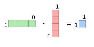
This is the intiutive explanation for why we do this. The technical answer lies in how we represent these matrices and how we have defined multiplication of matrices. Matrix multiplication is defined as each row of the first matrix being multiplied with each column of the second one. This is shown below:
Also, we represent a standard translation matrix as : $(M_{T}) = \begin{bmatrix}1 & 0 & D_{x} \\ 0 & 1 & D_{y}\\ 0& 0 & 1\end{bmatrix}$
If instead, we represented it as $(M_{T}) = \begin{bmatrix}1 & 0 & 0 \\ 0 & 1 & 0\\ D_{x}& D_{y} & 1\end{bmatrix}$, then we would not need to premultiply.
Hence, it is just a matter of technical representation and definition of matrix multiplication which leads to the need for premultiplication
Why are the last 3 elements 0, 0, 1 ?
We are interested to find the linear combination of the matrices. In a standard matrix multiplication for an equation like - $A*B=C$, then $A$ must be an $n × m$ matrix and $B$ must be an $m × p$ matrix. Their matrix product $C$ will be an $n × p$ matrix.
To facilitate linear multiplication of several transformation matrices, we add the third row with values $(0,0,1)$. This makes each matrix a $3 x 3$ square matrix which can be infinitely concatenated with other $3 x 3$ transformation matrices without losing its shape.
By doing this, we are essentially referring to a 3D space in which the transformations are happening. For the sake of convenience, a plane at $Z = 1$ is chosen, thus leading to the values $(0,0,1)$. Since the $X-Y$ plane itself is situated at $Z = 1$, its easy to see that any point $(x, y)$ in the $X-Y$ plane will be $(x, y, 1)$ in the 3D space.
Thus, finding point transformations is now simple. Let us consider the transformation matrix, $M = \begin{bmatrix}M_{11} & M_{12} & M_{13} \\ M_{21} & M_{22} & M_{23}\\ 0& 0 & 1\end{bmatrix}$ and find transformation for $(x, y)$.
$\begin{bmatrix}x \\ y \\ 1\end{bmatrix} * \begin{bmatrix}M_{11} & M_{12} & M_{13} \\ M_{21} & M_{22} & M_{23}\\ 0& 0 & 1\end{bmatrix} = \begin{bmatrix}x*M_{11} + y*M_{12} + M_{13} \\ x*M_{21} + y*M_{22} + M_{23} \\ 1\end{bmatrix} = \begin{bmatrix}x' \\ y' \\ 1\end{bmatrix}$
In this way, we can find the transformed point $(x', y')$